Implementing a dog bark detector

My dog has a little bit of separation anxiety so when we leave him alone, he barks some times.

We are training him to be home-alone and we want to know if he barks or not when we are not home.

Let’s implement a bark detector!

Basics

Time representation

What is audio and how is its digital representation? It’s basically an array of float values containing a value from -1 to 1.

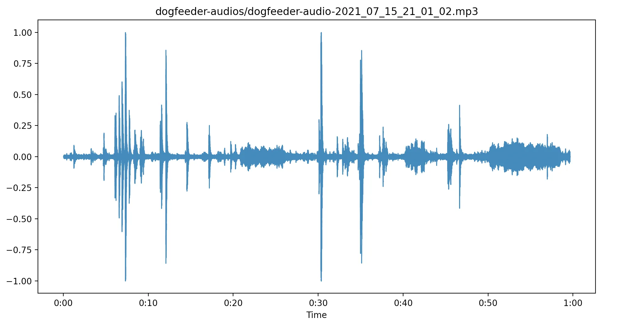
• Temporal representation of an audio signal

This representation shows the temporal evolution of the audio signal over time. This is very variable and it’s really difficult to extract any relevant feature from this representation.

Frequency representation

So, instead of using the temporal representation, let’s observe the frequency representation:

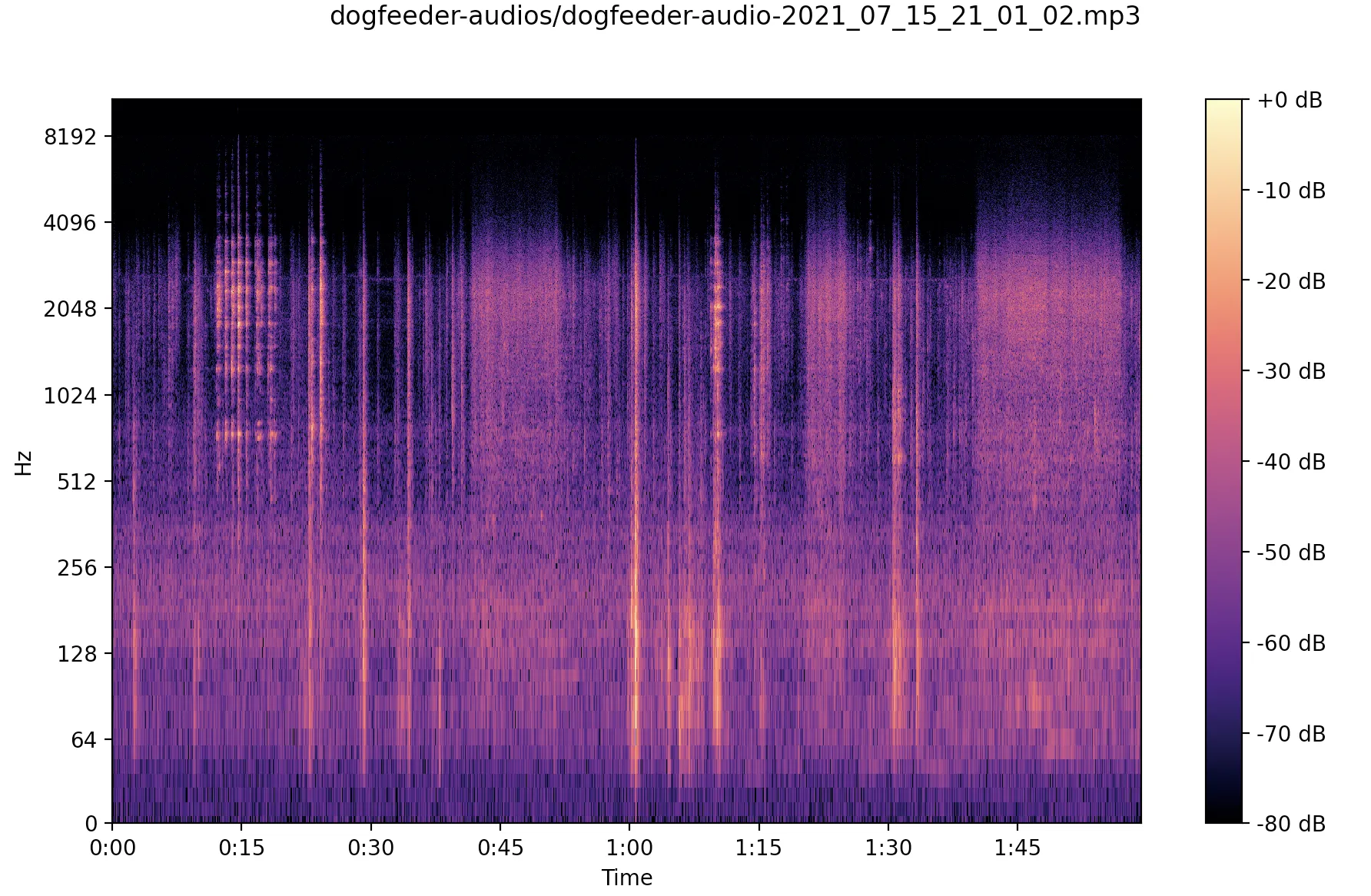
• Frequency representation of an audio signal

The x axis is the time of the audio signal and the y axis is the values of the frequencies. Each color in the vertical axis correspond to a different value of the power on that certain frequency.

Note that the time of the plot is doubled respect with the time representation, this is because the signal is combined with itself to generate the frequency representation.

This representation shows the evolution of the different frequency amplitudes over time.

Without even listening the sound, we can try to analise it checking the time/frequency characteristic. We see some peaks in the time representation that match with high energy in the low frequencies.

The good thing about frequency representation is that it cancel noise because usually its energy is spread over all frequencies. Besides that, each sound has a characteristic frequency footprint. So, it’s very convinient to extract the features of the sound in the frequency domain.

Mel Frequency Cepstral Co-efficients (MFCC)

Quoting from https://iq.opengenus.org/mfcc-audio/:

MFC is a representation of the short-term power spectrum of a sound, based on a linear cosine transform of a log power spectrum on a nonlinear mel scale of frequency.

Ok, what does it mean? It’s an improved frequency representation but applying optimizations based on the characteristics of human hearing. Usually MFCC are obtained like this:

1. Take the Fourier transform of the audio signal to get the frequency representation.
2. Map the powers of the spectrum to the mel scale. This scale approximates the spectrum to be more like what humans hear.
3. Take the logs of the powers at each of the mel frequencies.
4. Take the discrete cosine transform (DCT) of the list of mel log powers. This will remove redudant information as in non-changing information.
5. The MFCCs are the amplitudes of the resulting spectrum.

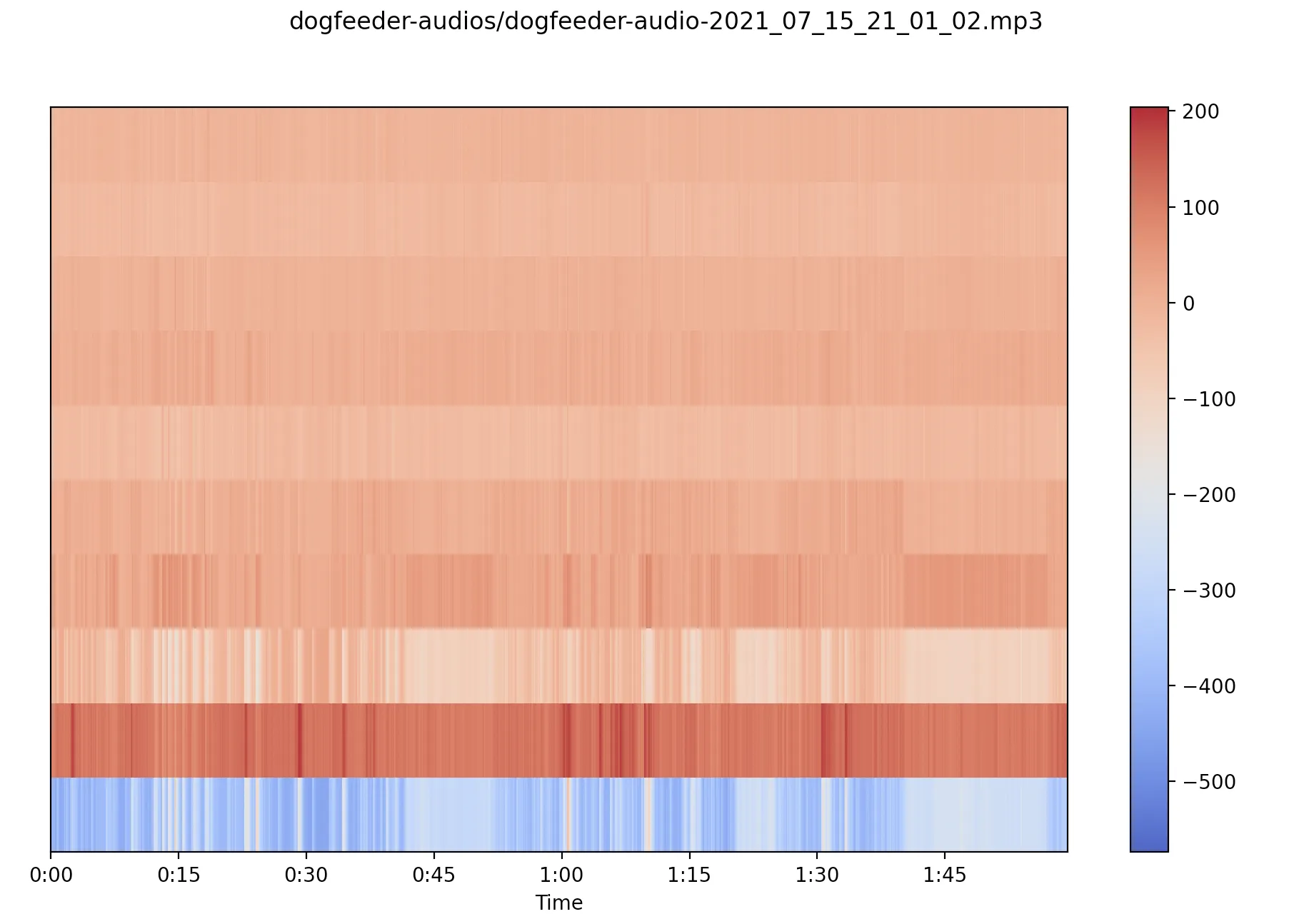
• MFCC representation of an audio signal

We can use librosa library to load the audio and extract the MFCC features.

The x axis is time, the y axis is the different MFCC coefficients computed (20 in this example). The color shows the value MFCC coefficient for certain time and coefficient.

It’s not obvious to see anything in this plot, but it represents the frequency information in a format the computer can use to understand the characteristics of this sound.

Getting the dataset

In this article I describe the little device I made to feed my dog while I’m away. So I’ll re-use the same device and plug it an old unused webcam that has a microphone.

I did not want to complicate my life much and I created a simple script that uses vlc to stream the audio obtained by the webcam mic and store it as mp3. In order to analyse the files easier I run the script every minute so I have recordings of 60 seconds duration:

#!/bin/bash
TIMEOUT=60
FILE_NAME="/home/pi/dogfeeder-audios/dogfeeder-audio-$(date +'%Y_%m_%d_%H_%M_%S').mp3"
timeout "$TIMEOUT" cvlc --no-video alsa://plughw:1 --sout="#transcode{vcodec=none,acodec=mp3,ab=128,
channels=2,samplerate=44100}:duplicate{dst=std{access=http,mux=mp3,dst=:8087},dst=std{access=file,mux=wav,
dst=$FILE_NAME}}" &

The syntax of vlc is really ugly :( . But if you read it carefully, you will see that we’re telling vlc to transcode the audio coming from alsa://plughw:1 device (webcam microphone) to mp3 at 128 kbps (decent compression rate). After that, stream the generated mp3 via HTTP on port 8087 and store the mp3 data on the given filename.

In order to don’t flood the SD card of the Raspberry Pi I run the following script each 15 minutes. It gets the files older than 15 minutes, copy them to a NAS and remove them from the Raspberry Pi disk.

#!/bin/bash
MINUTES_ALLOWED=15
FILES_TO_DELETE=$(find /home/pi/dogfeeder-audios -type f -mmin +"$MINUTES_ALLOWED" -exec ls {} +)

for file in $FILES_TO_DELETE; do
    scp "$file" admin@diskstation.local:/volume1/data/dogfeeder-audios/.
    rm "$file"
done

Training the model

I’ve been recording for 3 days and we made some exits to keep him alone. Up to this point we have enough data to train the model. However, we have 60 min * 24 h * 3 days = 4320 files and need to classify them manually. Will we do that manually? Absolutely not!

We can pre-process the dataset and check for files that have something different than noise.

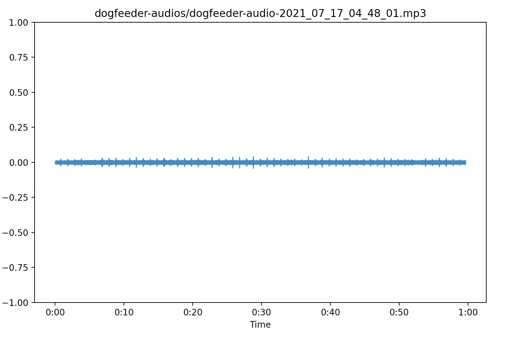
• File with only noise

• File with unclassified audio event

Since my dog’s barks are quite loud we can safely discard all files whose maximum amplitude is lower than 0.25. This way, we could reduce a lot the amount of files that need to be manually classified as bark.

Characterization of a bark

As mentioned before, we’ll discard files whose amplitude is lower than 0.25. Listening to multiple files with bark, we can observe that each bark more or less lasts for 1 second.

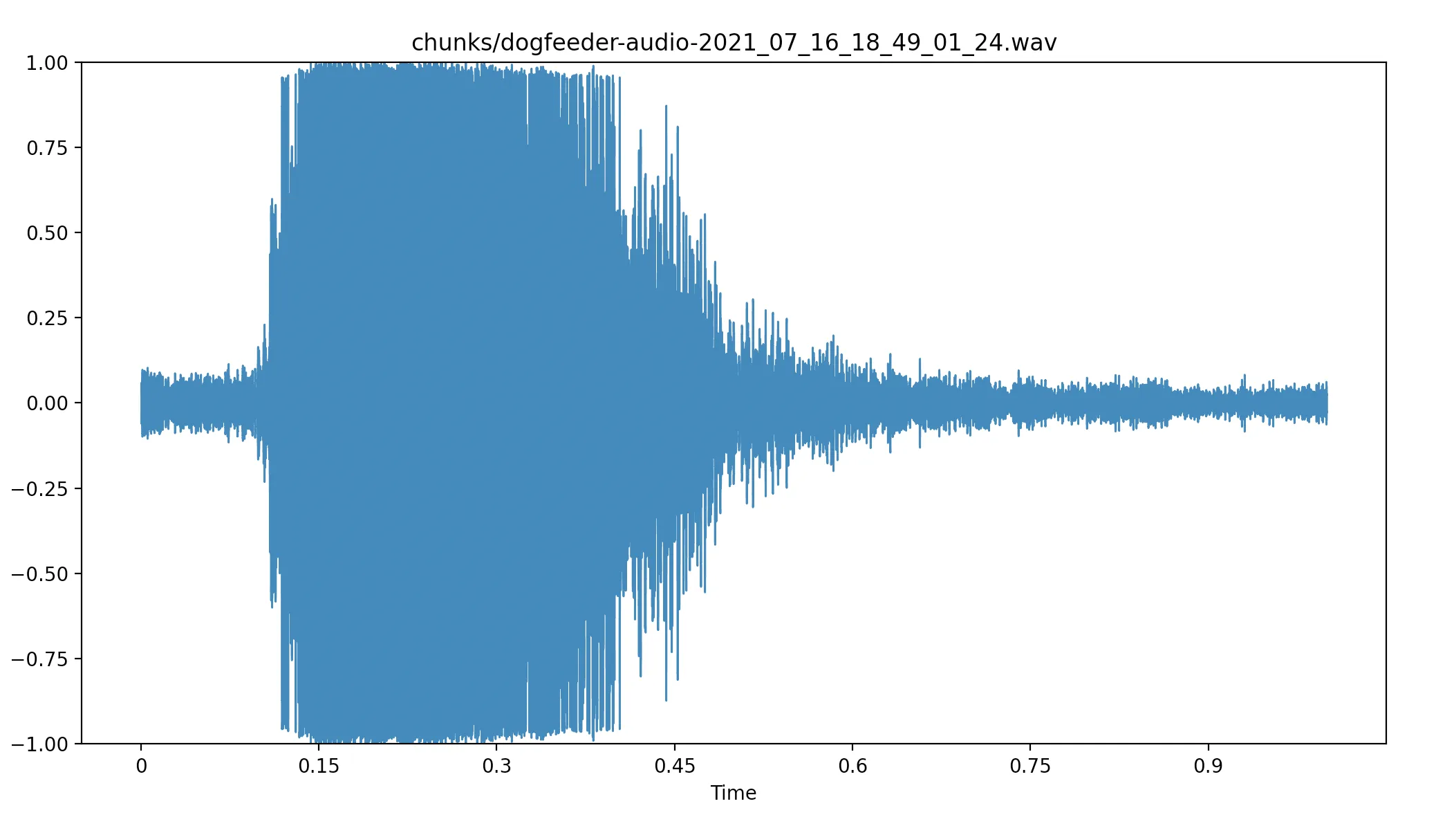
• Time representation of an audio signal containing a bark

Labelling the dataset

So, the strategy for labelling the dataset will be:

1. Download the whole dataset.
2. Discard the not interesting files (files without any sound event) by checking the maximum amplitude.
3. Extract chunks of 1 seconds from them, run again the algorithm to check sound events on the one-second chunks.
4. Manually listen to the chunks and classify them as bark or not. You can default the labelling to “Not Bark” and this way you only classify events that are barks.

The implementation of this is quite simple: write every chunk filename in a CSV and and a 0 or 1 signaling the presence of a bark or not:

chunks/dogfeeder-audio-2021_07_16_18_49_01_23.wav,0
chunks/dogfeeder-audio-2021_07_16_18_49_01_24.wav,1
chunks/dogfeeder-audio-2021_07_16_18_49_01_25.wav,0

Once we have the dataset labelled, we can go file by file and extract the MFCC features of every one-second file:

def extract_mfcc(filename):
    y, __ = librosa.load(filename, mono=True, sr=sample_rate)
    mfcc_2D = librosa.feature.mfcc(y, sr=sample_rate, n_mfcc=100)
    mfcc_1D = mfcc_2D.flatten()
    scaler = MinMaxScaler()
    mfccs_sc = scaler.fit_transform(np.array(mfcc_1D).reshape(-1, 1))
    return mfccs_sc.flatten()

MFCC values can go from [-Inf, Inf], however when I was playing with different algorithms, some of them did not accept negative values, so I scaled the values of MFCC to [0, Inf] using MinMaxScaler.

Once we have the MFCC features for all the dataset, we can split the dataset into training and test dataset using:

from sklearn.model_selection import train_test_split
X_train, X_test, y_train, y_test = train_test_split(
        X, Y, random_state=42, test_size=0.33)

After that, I’ve assesed the prediction performance of Naive Bayes classifier and Logistic Regression classifiers:

    # Naive bayes
    print("Training naive bayes ...")
    mnb = MultinomialNB().fit(X_train, y_train)
    print("score on test: " + str(mnb.score(X_test, y_test)))
    print("score on train: " + str(mnb.score(X_train, y_train)))
    print("***************")

    # Logistic regression
    print("Training logistic regression ...")
    lr = LogisticRegression(max_iter=1000)
    lr.fit(X_train, y_train)
    print("score on test: " + str(lr.score(X_test, y_test)))
    print("score on train: " + str(lr.score(X_train, y_train)))

Getting a very good score with the logistic regression, I don’t remember exactly the numbers but were more or less:

• Score on test: 0.992
• Score on traing: 0.996

Dataset imbalance

The number of events with barks will be very reduced compared with the events that does not contain a bark. This can present a huge problem depending on the machine learning algorithm returning a totally biased model.

In order to fix that, you can do two things:

1. Oversample: create positive samples by synthetically creating new positive samples
2. Undersample: discard samples from the negative ones

More info: https://towardsdatascience.com/having-an-imbalanced-dataset-here-is-how-you-can-solve-it-1640568947eb

I’ve used SMOTE (Synthetic Minority Over-sampling Technique) technique to perform the oversampling with very satisfactory results. In simple terms, SMOTE looks at the feature space for the minority class data points and considers its k nearest neighbours.

To do that I’ve used imbalanced-learn python libary and it’s really simple:

def fix_imbalance(X, Y):
    over = SMOTE(sampling_strategy=0.1)
    under = RandomUnderSampler(sampling_strategy=0.5)
    steps = [('o', over), ('u', under)]
    pipeline = Pipeline(steps=steps)
    X_fix, Y_fix = pipeline.fit_resample(X, Y)
    return X_fix, Y_fix

Note that the library also provides a module to perform majority under sampling. The two methods are combined in a pipeline to fix the dataset imbalance problem.

Using the training model

Now we have our logistic regression model trained and is working quite well. It’s time to put it on the Raspberry Pi.

First of all, we need a way to export the model outside of the training python code. In order to do that, I use the joblib library:

# Write the model
lr = LogisticRegression(max_iter=1000)
lr.fit(X_train, y_train)
joblib.dump(lr, 'lr.pkl', compress=9)

joblib serialize the object into that file and then Raspberry Pi can load the model object:

model = joblib.load('lr.pkl')

Now we can retrieve the more recent fully recorded audio file:

def last_fully_written_file():
    return audios_path + "/" + sorted(os.listdir(audios_path))[-2]

If the script query the last file, it might happen that is not fully written by that time.

Split it into chunks of one second and for each chunk run the prediction:

def has_bark_in_minute(filename):
    model = joblib.load('lr.pkl')

    audio_data, __ = load_audio_from_file(filename)
    chunks = split_in_one_second_chunks(audio_data, sample_rate)
    chunk_predictions = []
    for chunk in chunks:
        if len(chunk) == sample_rate:
            mfccs = extract_mfcc(chunk)
            chunk_predictions.append(model.predict(np.array([mfccs]))[0])

    return chunk_predictions.count(1) > 2, chunk_predictions

Since the model is probabilistic, it might happen to have false positive or negatives. In order to avoid that, the function has_bark_in_minute will only return True when more than two barks are detected for one minute.

Last but not least, when a bark is detected, the script will send me a message over telegram:

def send_to_telegram(predictions, filename):
    date = filename.split("-")[-1].split(".mp3")[0]

    welcome_msg = f"Detected {predictions.count(1)} barks on {date}"

    response = requests.post(
        f"https://api.telegram.org/bot{get_token()}/sendMessage",
        data={"chat_id": telegram_group_id, "text": welcome_msg},
    )
    print(response.text)